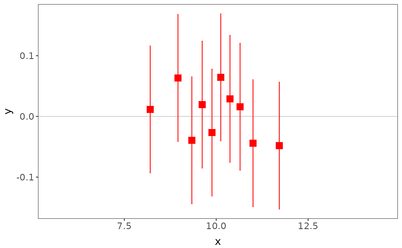
mvshape_plot — mvshape_plot • mvshape

mvshape_plot plots the meta-analysis results against the mean values of the exposure in each group.

Usage

mvshape_plot(
  mvshape,
  logx = FALSE,
  logy = FALSE,
  pref_x = "x",
  pref_y = "y",
  xbreaks = NULL,
  ybreaks = NULL,
  betacolour = "red",
  cicolour = "red",
  intcolour = "grey",
  xlim = NULL
)

Arguments

mvshape: a mvshape object.
logx: plot the x-axis on the log-scale.
logy: plot the y-axis on the log-scale.
pref_x: the prefix for the x-axis.
pref_y: the prefix for the y-axis.
xbreaks: breaks in the x-axis.
ybreaks: breaks in the y-axis.
betacolour: colour of the regression line.
cicolour: colour of the 95% confidence intervals.
intcolour: colour of the intercept line.
xlim: x-axis limits.

Value

mvshape plot.

Author

James Staley jrstaley95@gmail.com

Examples

# Data
y <- rnorm(5000)
x <- rnorm(5000, 10, 1)
c1 <- rbinom(5000, 1, 0.5)
c2 <- rnorm(5000)
study <- c(rep("study1", 1000), rep("study2", 1000), rep("study3", 1000), rep("study4", 1000), rep("study5", 1000))
covar <- data.frame(c1 = c1, c2 = c2, study = study)

# Analyses
res <- mvshape(y = y, x = x, covar = covar[, c("c1", "c2")], study = study, family = "gaussian")
mvshape_plot(res)